Immutable data structures

I already discussed that all data structures in purely functional programs are immutable; see Lecture 1. In this lecture, I will introduce some examples of immutable data structures that can be used as alternatives to common mutable data structures from imperative programming languages. It is beyond this introductory course to study immutable data structures in detail. I hope these examples will give you a brief insight into the topic.

From the general perspective, we distinguish two kinds of data structures:

• Immutable (aka persistent) data structures cannot be changed during their existence. Their advantage is that they can be safely shared between several data structures or concurrent threads. On the other hand, immutable data structures often have worse complexity bounds than their mutable equivalents. For example, we can look up an element stored in a mutable array at a given index in constant time . The same operation over an immutable array usually works in logarithmic time with respect to the array size .
• Mutable (aka ephemeral) data structures can be modified, but their previous versions are lost. They have better complexity bounds. On the other hand, they cannot be safely shared as the shared part might be mutated.

To illustrate the issues with sharing mutable data, consider the following code in Racket:

(define x '(0 1 2 3 4))
(define y (cdr x))

We defined a list x consisting of five elements. As Racket lists are immutable, we can safely share their content. Thus the defined list y shares all its members with x.

On the other hand, consider the same situation in Python:

x = [0,1,2,3,4]
y = x[1:]

As Python lists are mutable, y cannot share its content with x because x might be later modified. For example, y[0] equals 1 even after modifying x as follows:

x[1] = 333

Consequently, to create y, we must copy all the elemets from x[1:].

Lists

Before I describe some clever immutable data structures, I will focus on how immutability affects lists which are fundamental data structures for Racket. Recall that lists are built out of pairs whose first component carries data and the second component contains the continuation of the list. Internally, the second component is a pointer to the next pair. In other words, lists are stored as singly linked lists. Consequently, we can easily extract the first element and add a new element at the beginning of the list. More precisely, we can do it in constant time . On the other hand, appending a new element to the end of the list needs linear time where is the length of the list. Similarly, extracting the element at a given position or modifying it also requires linear time .

Let us see in more detail what happens if we concatenate two lists. Appending a list ys to a list xs, requires linear time in the length of xs. The append function can be implemented in Racket as follows:

(define (my-append xs ys)
  (if (null? xs)
      ys
      (cons (car xs) (my-append (cdr xs) ys))))

If xs is empty, there is nothing to do. The result is ys. Otherwise, we append recursively ys to (cdr xs) and prepend (car xs) to the result of the recursive call. The function my-append above is not tail recursive. I chose this version because it is conceptually simple and better for further explanation. If you wonder how to implement append as a tail-recursive function, you can check it below:

(define (my-append-tailrec xs ys)
  (define (iter l acc)
    (if (null? l)
        acc
        (iter (cdr l) (cons (car l) acc))))
  (iter (reverse xs) ys))

Now return to the first implementation of my-append. To practice pattern matching, let me reimplement it via match:

(define (my-append xs ys)
  (match xs
    [(list) ys]
    [(list x us ...) (cons x (my-append us ys))]))

Suppose we append a list ys to a list xs and name the resulting list zs:

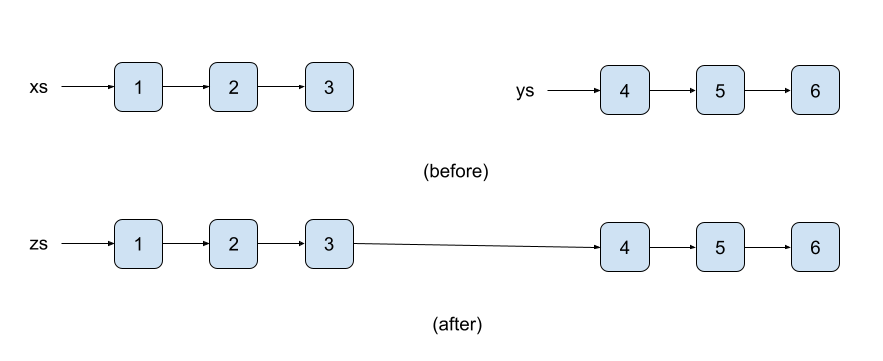
(define zs (my-append xs ys))

What happens is that xs is recursively decomposed and copied so that its copied version is connected to ys. The situation is depicted below on three-element lists '(1 2 3) and '(4 5 6).

Both original lists xs and ys are persistent, i.e., none is destroyed. Moreover, ys shares its members with the resulting list zs. This contrasts with the imperative setting where appending might be destructive. Updating the second component of the last pair in xs so that it points to ys, destroys the original xs as we do not know where it ends.

An analogous situation occurs if we need to modify an element at a given position in a list. It requires linear time because we must copy all the list members before the modified element.

(define (my-list-set lst pos val)
  (match (cons lst pos)
    [(cons (list) _) (error "Incorrect index")]
    [(cons (list _ xs ...) 0) (cons val xs)]
    [(cons (list x xs ...) i) (cons x (my-list-set xs (- i 1) val))]))

 (my-list-set (range 10) 4 'a) => '(0 1 2 3 a 5 6 7 8 9)

Note in the above code that we need to match against the given list and position. Thus we make a pair from the list and position and match the pair (Line 2). Modifying the empty list leads to an error (Line 3). If the -th element should be modified, we cons it to the remaining elements xs (Line 4). Otherwise, x is copied and consed to the result of the recursive call (Line 5).

Queues

Queues are common data structures representing a buffer. It stores data in the order they are coming in and releases the first-coming elements first. A queue is usually endowed with two operations: enqueue and dequeue. The first adds new-coming data to the back of the queue. The second removes the data stored in the front.

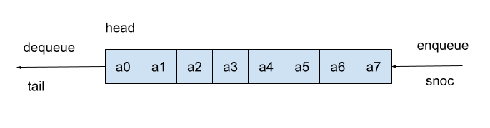
Following the tradition of functional programming, I will call enqueue and dequeue, respectively, snoc and tail. snoc is cons spelled backward, so its name should express that it adds an element to the back of the queue. Apart from snoc and tail, I also implement the function head reading the first element of the queue.

The question is how to implement queues in a purely functional language. A naive solution would use just lists as follows:

(define naive-head car)
(define naive-tail cdr)
(define (naive-snoc x q) (append q (list x)))

Note that naive-snoc applies the function append, which requires time . Consequently, this implementation is inefficient. How can we improve snoc in the purely functional setting if we cannot modify the pair holding the last element of the queue? The idea is simple. We will represent a queue via two lists: the front list and the rear list.

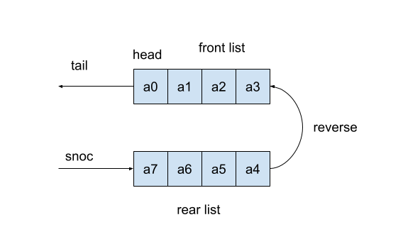
We strip off the first element from the front list to dequeue an element. It can be done in constant time . Analogously, to enqueue an element, we prepend it to the rear list. This can be done in as well. Obviously, the members of the rear list are ordered reversely. The only issue is transferring data from the rear list to the front one. The simplest variant maintains an invariant that the front list is always non-empty unless the whole queue is empty. This means that once we dequeue all data from the front list, we make a new front list from the reversed rear list. The reversing operation needs linear time . Thus the worst-case time complexity for dequeuing is . However, the amortized time complexity is . The amortized time complexity means how the algorithm behaves on average. Even though dequeuing could sometimes take linear time , there must be sufficiently many dequeuing steps working in constant time . These fast steps compensate for the expensive reverse operation.

The implementation of the improved queue in Racket is below:

(struct queue (front rear) #:transparent)

(define empty-queue (queue '() '()))

(define (queue-empty? q) (null? (queue-front q)))

(define (check q)
  (if (null? (queue-front q))
      (queue (reverse (queue-rear q)) '())
      q))

(define head (compose car queue-front))

(define (snoc x q)
  (check (queue (queue-front q) (cons x (queue-rear q)))))

(define (tail q)
  (check (queue (cdr (queue-front q)) (queue-rear q))))

We represent the queue as a structure with two components: the front and rear list (Line 1). The empty queue consists of two empty lists (Line 3). The implementation maintains the invariant that the queue is empty if, and only if, the front is empty. Thus to test if the queue is empty, we check if the front list is empty (Line 5). The function check (Line 7) maintains the invariant. If the front list is empty (Line 8), we create a new queue whose front list is the reverse of the rear list, and the rear is empty (Line 9). If the front list is non-empty, we return the input queue q (Line 10).

Now the main functions. head simply extracts the first element of the front list (Line 12). snoc creates a new queue whose front list is preserved, and the rear list is expanded by the new element x (Line 15). Moreover, we must check if the invariant holds. In fact, the only case when the invariant might be invalid is when we snoc a new element into the empty queue. Similarly, tail removes the first element of the front list and checks the invariant (Line 18).

Let us see how the improved queue works. If we enqueue a symbol 'a to the empty queue, it inserts 'a into the rear list. As the front list is empty, the function check reverses the rear list and makes it the front list.

(snoc 'a empty-queue) => (queue '(a) '())

If we continue adding new elements into the queue, they are consed to the rear list.

(snoc 'c (snoc 'b (snoc 'a empty-queue))) => (queue '(a) '(c b))

Once we dequeue the first element, the front list becomes empty again, so check must fix the invariant by reversing the rear list.

(tail (snoc 'c (snoc 'b (snoc 'a empty-queue)))) => (queue '(b c) '())

If we add further elements, they are consed to the rear list.

(snoc 'd (tail (snoc 'c (snoc 'b (snoc 'a empty-queue))))) => (queue '(b c) '(d))

Now we can compare the performance of the naive queue and the improved one. To test the performance, we generate a list of random queue commands consisting either of the symbol 'tail or a symbol to be enqueued.

(define (make-data n)
  (define rnd-lst (map random (make-list n 2)))
  (define (generate-event k)
    (match k
      [1 (gensym)]
      [0 'tail]))
  (map generate-event rnd-lst))

Line 2 generates a random sequence of zeros and ones. The function generate-event (Lines 3-6) converts zeros to 'tail and ones to fresh symbols (they can be generated by gensym). Finally, Line 7 creates testing data. The output of make-data might look as follows:

(make-data 10) =>
'(g6642396 g6642397 g6642398 tail tail g6642399 g6642400 g6642401 g6642402 tail)

Next, we need a function applying the testing data to a particular queue.

(define (test-data q0 empty? enq deq data)
  (define (exec cmd q)
    (match cmd
      ['tail (if (empty? q) q (deq q))]
      [el (enq el q)]))
  (foldl exec q0 data))

The function test-data accepts an initial queue q0, a predicate testing queue's emptiness empty?, functions enq and deq enqueuing and dequeuing an element, and testing data. The local function exec (Lines 2-5) executes a command cmd on the queue. If cmd is 'tail, the first element is dequeued provided the queue is non-empty. Otherwise, cmd is an element to be enqueued. Line 6 runs all the commands on the initial queue q0.

Now it remains to measure the times needed to evaluate test-data. We first create testing data data and then compare the performance. To prevent displaying the large queues on the screen, we can enclose the call of test-data inside begin and returns just a value 'done.

(define data (make-data 1000000))
(time (begin (test-data empty-queue queue-empty? snoc tail data) 'done))
(time (begin (test-data '() null? naive-snoc naive-tail data) 'done))

cpu time: 62 real time: 64 gc time: 31
'done
cpu time: 1718 real time: 1769 gc time: 218
'done

The first time corresponding to the improved queue is considerably shorter than the second one corresponding to the naive implementation.

Random access lists

Arrays are the most common data structures in imperative programming. An array is a collection of indexed elements that can be quickly accessed and updated, i.e., in constant time . If we restrict ourselves to pure functional programming, inventing a data structure behaving like an array with a fast lookup and update is not so easy. In this section, I will discuss such a data structure called a random access list. It behaves like a list with lookup and update operations whose running times are, in worst-case, logarithmic . Several variants of random access lists are already implemented in Racket; see the documentation. I will implement the simplest variant called Binary random access lists.

Analogously to queues, one can naively implement arrays as lists. However, as we already know, the lookup and update operations run in linear time for lists. A usual approach to overcome this issue is to represent arrays as self-balancing trees (e.g., AVL trees or Red-black trees). Then the lookup can be done in the logarithmic time because such a tree's height is logarithmic in size. The self-balancing mechanism is usually quite complicated. Thus, I will discuss Binary random access lists for their simplicity.

The problem with the regular list is that their length equals their size. Thus, it takes a linear time if we want to iterate through them to look up an element. To overcome this, we can split the list's members into chunks so that there are only logarithmically many chunks. The way we create the chunks is based on the binary numeral system. Recall that every number can be uniquely represented as follows: [n=b_0\cdot 2^0 + b_1\cdot 2^1 + b_2\cdot 2^2 + \cdots + b_k\cdot 2^k ] where are the bits of its binary representation; is the least significant bit and the most significant. Assuming that the most significant bit , we have , implying . In other words, the number of bits we need to represent is logarithmic.

Suppose we want to represent an array of size . For each non-zero bit , we create a chunk of elements. These chunks altogether give us the whole array. For example, if [n=10=1\cdot 2^1 + 1\cdot 2^3,] we split the elements into two chunks; the first of size and the second of size .

As the chunks are of size , i.e., still too large to be processed as regular lists, we represent them as leaves of a complete binary tree. Thus we can quickly look up an element inside a chunk.

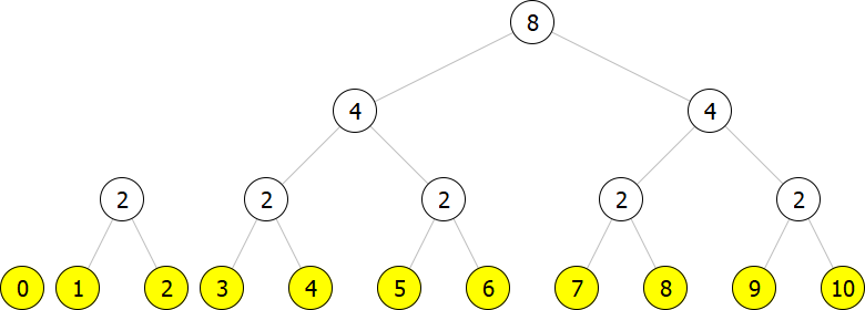
Altogether, we represent an array of size as a list of complete binary trees of size for s such that . Consider, for instance, an array of size . Its representation is a list of two trees depicted below:

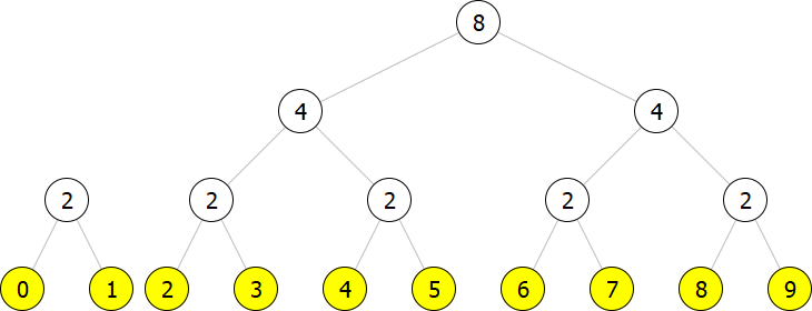
The chunks corresponding to non-zero bits are the binary trees. Their leaves (yellow nodes) hold the data. For convenience, the inner nodes (white nodes) contain information about the number of leaves below them.

Now we can discuss how to implement this representation in Racket. We define two structures—one for the inner nodes and the other for the leaves.

(struct node (size left right) #:transparent)
(struct leaf (val) #:transparent)

Thus the inner node is a triple consisting of the number of leaves below it and left and right subtrees. The leaf contains only a value. So the above-depicted list of trees is represented in Racket as follows:

(list (node 2 (leaf 0)
              (leaf 1))
      (node 8 (node 4 (node 2 (leaf 2)
                              (leaf 3))
                      (node 2 (leaf 4)
                              (leaf 5)))
              (node 4 (node 2 (leaf 6)
                              (leaf 7))
                      (node 2 (leaf 8)
                              (leaf 9)))))

Next, we need to deal with a function building random access lists. In particular, we will implement a function cons-el, adding one new element to an existing random access list. Adding a new element to a random access list of size follows the standard procedure of adding to in binary representation. This standard procedure adds to . If , we set , and we are done. If , then and we carry to the next bit, and the process continues. For example, for [n=11=1\cdot 2^0+1\cdot 2^1+0\cdot 2^2 + 1\cdot 2^3,] we get [n+1=12=0\cdot 2^0+0\cdot 2^1+1\cdot 2^2+1\cdot 2^3.] Thus we carry twice until we encounter , the bit whose weight is .

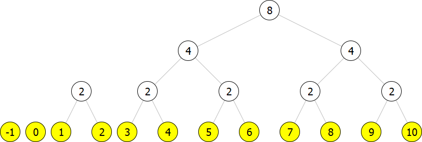
Let us see how the binary increment by influences the structure of random access lists. An array consisting of elements is represented as follows:

Now we add a new element, say , as (leaf -1).

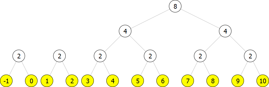
However, this is not a correct representation because we have two trees of size . Thus we need to join them and create a new tree of size .

The result is still not a correct representation as we have two trees of size . Thus we must join them again.

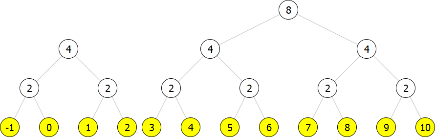
Now we have a correct representation for the array of size .

To compare the sizes of trees, we need a helper function returning the size of a tree/chunk, i.e., the number of leaves in a tree.

(define (size t)
  (match t
    [(node w _ _) w]
    [(leaf _) 1]))

The function size matches the root node of the input tree. If it is a leaf, then the size is . Otherwise, the size is extracted from the root node.

Further, it is necessary to implement a function joining two trees of sizes and returning a tree of size .

(define (link t1 t2)
  (node (+ (size t1) (size t2)) t1 t2))

The function link joins two trees and adds a new root node with the sum of their sizes.

The following function cons-el inserts an element into a random access list lst.

(define (cons-el el lst)
  (cons-tree (leaf el) lst))

(define (cons-tree t lst)
  (match lst
    [(list) (list t)]
    [(list t2 ts ...)
     (if (< (size t) (size t2))
         (cons t lst)
         (cons-tree (link t t2) ts))]))

The element is added to lst as a tree (leaf el) of size via a recursive helper function cons-tree (Line 2). The helper function inserts a tree t into lst. It matches lst and, based on its structure, decides how to insert t. If lst is empty (Line 6), we return a singleton list containing only t. If lst is non-empty (Line 7), we extract its first tree t2. We must compare the sizes of t and t2 (Line 8). When t is strictly smaller than t2, we simply cons t to lst (Line 9). We can do that because no tree in lst has the same size as t. Otherwise, the sizes must be equal. Thus we must join the trees and recursively insert the joined tree (Line 10).

Let us see the first few calls of cons-el if we build a random access list from the empty one.

(cons-el 'a '()) => (list (leaf 'a))

(cons-el 'b (cons-el 'a '())) => (list (node 2 (leaf 'b)
                                               (leaf 'a)))

(cons-el 'c (cons-el 'b (cons-el 'a '()))) => (list (leaf 'c)
                                                    (node 2 (leaf 'b)
                                                            (leaf 'a)))

(cons-el 'd (cons-el 'c (cons-el 'b (cons-el 'a '())))) =>
(list (node 4 (node 2 (leaf 'd)
                      (leaf 'c))
              (node 2 (leaf 'b)
                      (leaf 'a))))

Inserting the first element 'a creates a list containing only (leaf 'a) (Line 1). Adding the second element 'b must join two leaves; thus we end up with a single binary tree of size (Lines 3-4). The third element 'c is included as (leaf 'c) (Lines 6-8). Finally, inserting the forth element 'd' results in a single tree of size (Lines 11-14).

One can also implement a function tail removing the first element from a given random access list lst. It extracts the first tree/chunk t from lst and removes its first element by the function tail-tree. If t is a leaf, we just discard it. Otherwise, we split the tree into the left and right subtrees. The right subtree is preserved, and we recursively remove the first element from the left subtree.

(define (tail lst)
  (match lst
    [(list) (error "empty list")]
    [(list t ts ...) (tail-tree t ts)]))

(define (tail-tree t ts)
  (match t
    [(leaf _) ts]
    [(node _ t1 t2) (tail-tree t1 (cons t2 ts))]))

Now, we know how to build random access lists. The next question is how to implement the lookup and update functions running in logarithmic time. We assume that elements stored in a random access list are indexed from zero. The function lookup extracts the element from a given random access list lst whose index is i. It must first identify the right chunk/tree where the element is stored.

(define (lookup i lst)
  (match lst
    [(list) (error "incorrect index")]
    [(list t ts ...)
     (define s (size t))
     (if (< i s)
         (lookup-tree i t)
         (lookup (- i s) ts))]))

We throw an error if lst is empty (Line 3). Otherwise, we extract the first chunk/tree t and the rest ts (Line 4). If the index i is smaller than the size of t (Line 6), we know the element we seek is inside t. So we extract it by calling a helper function lookup-tree (Line 7). If i is greater than or equal to the size of t, we know that the element is not in t. Thus we subtract from i the size of t and recursively look up in the remaining chunks/trees ts (Line 8).

The following helper function looks up an element inside a given chunk/tree t whose index is i.

(define (lookup-tree i t)
  (match (cons i t)
    [(cons 0 (leaf x)) x]
    [(cons _ (leaf _)) (error "incorrect index")]
    [(cons i (node w t1 t2))
     (define half (quotient w 2))
     (if (< i half)
         (lookup-tree i t1)
         (lookup-tree (- i half) t2))]))

The -th element in a leaf is the element stored in that leaf (Line 3). Leaves contain no elements of non-zero indexes (Line 4). If the size of t is greater than , we extract the size w of t and its left and right subtrees t1 and t2 (Line 5). We divide w by two to determine if the sought element is in the left or right subtree (Lines 6-7). Lines 8-9 recursively call lookup-tree again.

Note that lookup runs in logarithmic time in size of the random access list. To see that, observe that there are only logarithmically many trees/chunks. Thus it takes steps to find the right tree/chunk. Next, the elements are stored in complete binary trees. Thus it again requires steps to locate the desired element inside a tree/chunk. Altogether, we need twice steps, which is just .

The update function is analogous to the lookup function. The only difference is that we must build the updated random access list.

(define (update i y lst)
  (match lst
    [(list) (error "incorrect index")]
    [(list t ts ...)
     (define s (size t))
     (if (< i s)
         (cons (update-tree i y t) ts)
         (cons t (update (- i s) y ts)))]))

(define (update-tree i y t)
  (match (cons i t)
    [(cons 0 (leaf _)) (leaf y)]
    [(cons _ (leaf _)) (error "incorrect index")]
    [(cons i (node w t1 t2))
     (define half (quotient w 2))
     (if (< i half)
         (node w (update-tree i y t1) t2)
         (node w t1 (update-tree (- i half) y t2)))]))

Note Lines 7-8; they build the updated random access list. If the modified element is not in the current tree/chunk t, we cons t to the result of the recursive call (Line 8). Otherwise, we update t by the function update-tree (Line 7). Similarly, update-tree is analogous to lookup-tree. Lines 17-18 do the update. If the modified element is in the left subtree, we update only the left subtree and keep the right one untouched (Line 17). Line 18 analogously updates only the right subtree.

The complexity analysis of update is the same as for lookup, i.e., .

Let us check how update works:

(define ral (cons-el 'c (cons-el 'b (cons-el 'a '()))))

ral => (list (leaf 'c)
             (node 2 (leaf 'b)
                     (leaf 'a)))

(update 1 333 ral) => (list (leaf 'c)
                            (node 2 (leaf 333)
                                    (leaf 'a)))

Now, let us compare the performance between the random access and regular lists. First, we define a function converting a standard list into a random access list.

(define (build-ra-lst lst)
  (foldl cons-el '() lst))

In our experiment, we create an array with ten million elements. Then we look up the last element and update it to the symbol 'a. The results for the random access lists are below:

(define ra-lst (time (build-ra-lst (range 9999999 -1 -1))))
(time (lookup 9999999 ra-lst))
(time (begin (update 9999999 'a ra-lst) 'done))

cpu time: 2781 real time: 2769 gc time: 2156
cpu time: 0 real time: 0 gc time: 0
9999999
cpu time: 0 real time: 0 gc time: 0
'done

Note that it took approximately 2.8s to build the random access list holding numbers from to . On the other hand, the times for lookup and update were negligible.

I used the standard built-in functions implemented in Racket to compare the results with the regular lists.

(define lst (time (range 10000000)))
(time (list-ref lst 9999999))
(time (begin (list-set lst 9999999 'a) 'done))

cpu time: 1468 real time: 1463 gc time: 1375
cpu time: 15 real time: 23 gc time: 0
9999999
cpu time: 2453 real time: 2449 gc time: 1234
'done

Note that creating a regular list of size ten million is faster than creating the random access list. On the other hand, the update is extremely slow.