Introduction to Haskell

Haskell is a pure, lazy ,and statically-typed functional programming language (as opposed to Racket which is eager and dynamically-typed).

Pure, in the context of Haskell, means that it is impossible to write mutating code. (Except for IO actions, which let us print to screen, but more on that in due time.)

Statically-typed: Haskell programs are checked and types derived at compile time. The type system is very powerful in Haskell and we will spend a lot of time learning about its different features/implications.

Lazy means that expressions are not evaluated until the are actually needed. This has far reaching consequences, for example we can easily deal with infinite data structures which enables programming in a very different style wholemeal programming^[1]. This approach enables much more modular code.

The interpreter - GHCi

The leading implementation of Haskell is the Glasgow Haskell Compiler (GHC). It includes both a compiler and an interpreter. GHC is written in Haskell (apart from small parts of the runtime in C/C--).

We will mostly be working with the interpreter GHCi:

$ ghci
GHCi, version 9.8.1: https://www.haskell.org/ghc/  :? for help
𝝺>

Like in the Racket REPL, you can evaluate Haskell expressions in this interpreter.

𝝺> fibs = 0 : 1 : zipWith (+) fibs (tail fibs)
𝝺> take 20 fibs
[0,1,1,2,3,5,8,13,21,34,55,89,144,233,377,610,987,1597,2584,4181]

The most important commands you can use in the REPL are

• :? for help
• :load <filename>
• :reload
• :type <expr> displays the type of and expr
• :info <name> displays info on a function or type
• :doc <name> displays documentation on a function or type
• :quit or ctrl-d

Custom REPL

To get the lambda prompt instead of Prelude> and also output type information automatically, you and use the following config:

$ cat ~/.ghc/ghci.conf
-- Enables type display
:set +t
-- Sets the prompt to a lambda
:set prompt "𝝺> "

Basic Syntax

This section covers some of the important features of Haskell including some notable differences of Haskell to Racket. It is not a complete description of the whole syntax of Haskell.

-- this is a comment

{-
this is a block comment
-}

x :: Int
x = 3

Above we defined a variable x with the Int and assigned the value 3 to it.

Every well-formed expression e has a well-formed type t written like e :: t:

𝝺> "a" ++ "b"
"ab"
it :: String

In the output above we concatenated two strings. The it is just Haskell's way of referring to the latest unnamed expression.

Haskell has a number of basic types, including:

• Bool: logical values True, False
• Char: single characters 'a'
• Strings of characters "abc"
• Int: fixed-precision integers
• Integer: arbitrary-precision integers
• Float: single-precision floating-point numbers
• Double: double-precision floating-point numbers

Functions

Function definitions have to start with a lower-case letter (like myFun, fun1, h', g_2, etc.) and we can do pattern matching on inputs (even integers):

factorial :: Int -> Int
factorial 0 = 1
factorial n = n * factorial (n-1)

Workflow

You can run the function above by copying the snippet above into a file (e.g. fact.hs), starting a REPL, and loading the file:

$ ghci
GHCi, version 9.8.1: https://www.haskell.org/ghc/  :? for help
𝝺> :load fact.hs
[1 of 2] Compiling Main             ( fact.hs, interpreted )
Ok, one module loaded.

Now the factorial function is available and we can call it

𝝺> factorial 5
120
it :: Int

Note, that we do not need parenthesis to make a function call. In fact, in Haskell, function application is denoted by a space ␣, so whenever you see expression like the following

f a b c

it describes a call to a function f that accepts three arguments a, b, and c.

In the first line of the factorial definition we are writing the function type signature. factorial is a function that accepts an Int and outputs an Int. Then we have two clauses (which are checked in the order they are written in and the first clause that matches a given input is used). Calling factorial 2 does not match the first clause, so the second one is used, because a variable (in this case n) matches anything. Hence, we end up with 2 * factorial (2-1), which can be further evaluated until we arrive at 2 * 1 * factorial 0, where we match the base case and end up with the final expression that is evaluated as soon as we want to print it.

To define functions of multiple variables, we just add them to the definition, for example

power :: Int -> (Int -> Int)
power _ 0 = 1
power n k = n * power n (k-1)

Note, that the type signature here hints at the fact that functions in Haskell are by default always curried!

We can define infix operators consisting only of special symbols, e.g. +/+ can be defined in infix notation:

x +/+ y = 2*x + y

An infix function can be turned into a prefix function by ( ):

𝝺> 2 +/+ 3
7
it :: Num a => a

𝝺> (+/+) 2 3
7
it :: Num a => a

We can also turn a prefix function into an infix function via `:

𝝺> elem 1 [2,1,3]
True
it :: Bool

𝝺> 1 `elem` [2,1,3]
True
it :: Bool

Local variables via let & where

Like in Racket we can use let:

discr :: Float -> Float -> Float -> Float
discr a b c =
    let x = b*b
        y = 4*a*c
    in x - y

or alternatively, we can use Haskell's where:

discr a b c = x - y
    where x = b*b
          y = 4*a*c

Layout rule

In Haskell, indentation matters, for example

a = b + c where
            b = 1
            c = 2

means

a = b + c where {b=1; c=2}

Keywords (such as where, let, etc.) start a block. The first word after the keyword defines the pivot column. Lines exactly on the pivot define a new entry in the block. You can start a line to the right of the pivot to continue the previous lines. Start a line to the left of the pivot to end the block.

Conditionals & Guards

Haskell has two way of express branching, the first is the classic if-then-else-clause:

abs n = if n>=0 then n else -n

You can of course nest these conditionals:

signum n = if n<0 then -1 else
             if n==0 then 0 else 1

You always have to provide an else branch. Additionally, the then-clause and the else-clause must have the same type!

𝝺> if True then 1 else "0" will throw an error.

𝝺> if True then 1 else "0"

<interactive>:1:14: error: [GHC-39999]
    • No instance for ‘Num String’ arising from the literal ‘1’
    • In the expression: 1
      In the expression: if True then 1 else "0"
      In an equation for ‘it’: it = if True then 1 else "0"

The error message above might seem a little daunting at first, but you will learn to handle them once you understand Haskell's type system a bit better. For now we can explain it as follows:

𝝺> if True then 1 else 2
1
it :: Num a => a

So Haskell expects the output type of the conditional to be some Number^[2] (could be Int, or Float, or something different). Now it received a String in the else-clause, so it tries to construct a Num String which is not possible.

As an alternative to conditionals, functions can also be defined using guards (which are similar to Racket's cond).

abs n | n >= 0 = n
      | otherwise = -n

Definitions with multiple conditions are then easier to read:

signum n | n < 0     = -1
         | n == 0    = 0
         | otherwise = 1

otherwise is defined in the prelude by otherwise = True.

Lists

Lists in Haskell, are very similar to Racket. They are singly linked lists, which are constructed via the operator : (equivalent to cons). They end with the empty list []. The important difference is that list elements have to have the same type, e.g. [Int].

Example lists

You can try an evaluate the following list expressions one by one and see what GHCi spits out:

𝝺> 1:2:3:4:5:[]
...

𝝺> [1..10]
...

𝝺> ['a'..'z']
...

𝝺> [10,9..1]
...

𝝺> [10,9..1]
...

𝝺> [1,3..]
...

Lists come with tons of predefined functions like take, length, ++, reverse, etc.

Hoogλe

Go an check out Hoogle in which you can search for all important Haskell functions. (You can even search for type signatures! - But more on those later.)

Functions on lists can be defined using x:xs patterns, for example:

𝝺> head (x:_) = x
𝝺> head [1,2,3]
1
it :: Num a => a

𝝺> tail (_:xs) = xs
𝝺> tail [1,2,3]
[2,3]
it :: Num a => [a]

We will see later it works similarly for other composite data types. The x:xs pattern matches only non-empty lists:

> head []
*** Exception: Non-exhaustive patterns in function head

The x:xs patterns must be parenthesised, because function application has higher precedence than (:). The following definition throws an error:

head x:_ = x

A part of the pattern can be assigned a name

copyfirst s@(x:xs) = x:s -- same as x:x:xs

Tuples

Tuples are fixed-size sequences of elements of arbitrary types, e.g. (Int, Char):

(1,2)
('a','b')
(1,2,'c',False)

Their element can be accessed by pattern matching

first (x,_,_) = x
second (_,x,_) = y
third (_,_,x) = x

Pattern matching can be nested

f :: (Int, [Char], (Int, Char)) -> [Char]
f (1, (x:xs), (2,y)) = x:y:xs

Comprehensions

In Haskell, there is a list comprehension notation to construct new lists from existing lists.

𝝺> [x^2 | x <- [1..5]]
[1,4,9,16,25]

x <- [1..5] is called a generator. Comprehensions can have multiple generators behaving like nested loops

𝝺> [(x,y) | x <- [1,2,3], y <- [4,5]]
[(1,4),(1,5),(2,4),(2,5),(3,4),(3,5)]

Generators can be infinite (almost everything is lazy)

𝝺> [x^2 | x <- [1..]]

Later generators can depend on the variables that are introduced by earlier generators.

𝝺> [(x,y) | x <- [1..3], y <- [x..3]]
[(1,1),(1,2),(1,3),(2,2),(2,3),(3,3)]

Using a dependent generator, we can define a function that concatenates a list of lists:

flatten :: [[Int]] -> [Int]
flatten xss = [x | xs <- xss, x <- xs]

𝝺> flatten [[1,2],[3,4],[5]]
[1,2,3,4,5]

List comprehensions can use guards to restrict the values produced by earlier generators.

[x | x <- [1..10], even x]

Using a guard we can define a function that maps a positive integer to its list of factors:

factors :: Int -> [Int]
factors n = [x | x <- [1..n], mod n x == 0]}

A prime’s only factors are 1 and itself

prime :: Int -> Bool
prime n = factors n == [1,n]

List of all primes

[x | x <- [2..], prime x]

Jarnik's Algorithm

To demonstrate a small, but complete program/algorithm in Haskell, we can implement Jarnik's Algorithm. It finds the minimum spanning tree of a weighted, undirected graph.

Jarnik's Algorithm as described on Wikipedia

1. Initialize a tree with a single vertex, chosen arbitrarily from the graph.
2. Grow the tree by one edge: Of the edges that connect the tree to vertices not yet in the tree, find the minimum-weight edge, and transfer it to the tree.
3. Repeat step 2 (until all vertices are in the tree).

To implement this algorithm we can first make use of Haskell's type system to define some type aliases that will make our code more readable:

type Vertex = Char
type Edge = (Vertex,Vertex)
type Weight = Int
type Graph = [(Edge,Weight)]

graph :: Graph
graph = [(('A','B'), 7)
        ,(('A','D'), 5)
        ,(('D','B'), 9)
        ,(('C','B'), 8)
        ,(('E','B'), 7)
        ,(('C','E'), 5)
        ,(('D','E'), 15)
        ,(('D','F'), 6)
        ,(('F','E'), 8)
        ,(('F','G'), 11)
        ,(('E','G'), 9)]

Before implementing the algorithm itself we will define a function vertices :: Graph -> [Vertex] which will give us all unique list of vertices in the graph. First, we collect all nodes from the graph

𝝺> [[a,b] | ((a,b),_) <- graph]
["AB","AD","DB","CB","EB","CE","DE","DF","FE","FG","EG"]

We concatenate all the strings into one and then deduplicate it:

𝝺> deduplicate (concat [[a,b] | ((a,b),_) <- graph])
"ABDCEFG"

deduplicate still has to be implemented:

deduplicate :: [Vertex] -> [Vertex]
deduplicate [] = []
deduplicate (v:vs) = v:(deduplicate filtered)
    where filtered = [ u | u <- vs, u /= v ]

where we used pattern matching to take out the first element of the list v, and filter the remaining list for v before consing (:). Now the vertices function can be written as:

vertices :: Graph -> [Vertex]
vertices g = deduplicate $ concat [ [a,b] | ((a,b), _) <- g ]

We will implement the algorithm based on a list of vertices to visit and a tree into which we will accumulate the edges of our spanning tree. For simplicity, this tree will just be a Graph again, but we will make sure it does not have any cycles. First, we will sort the Graph according to its Weights with the sortOn :: Ord b => (a -> b) -> [a] -> [a] function:

𝝺> sortOn snd graph
[ (('A','D'),5)
, (('C','E'),5)
, (('D','F'),6)
, (('A','B'),7)
, ... ]

Given the nodes to visit we need to find the next edge we want to put into our tree. Assuming we already went from A -> D, we will removed A and D such that

𝝺> vertices graph
"ABDCEFG"
𝝺> visit
"BCEFG"

The next edge has to have exactly one node in the nodes to visit:

checkEdge :: Edge -> [Vertex] -> Bool
checkEdge (a,b) visit = p /= q
    where p = a `elem` visit
          q = b `elem` visit

where `elem` is the infix version of elem :: a -> [a] -> Bool. Now, given a Graph that is sorted according to Weight, we can find the next edge by filtering:

𝝺> [(e,w) | (e,w) <- (sortOn snd graph), checkEdge e visit]
[ (('D','F'),6)
, (('A','B'),7)
, (('D','B'),9)
, (('D','E'),15) ]

Hence the next edge in the tree will be D -> F. We can wrap the above in a function:

findEdge :: [Vertex] -> Graph -> (Edge, Weight)
findEdge visit graph = head [(e,w) | (e,w) <- graph, checkEdge e visit]

Above we filter for the potential next edges and then take the first element with head. Now the only thing that remains to be done is iterate this function over the whole graph and maintain the visit and tree variables accordingly:

jarnik :: Graph -> Graph
jarnik graph = iter vs [] where
  graph' = sortGraph graph  -- sort the graph once in the beginning
  (_:vs) = vertices graph   -- all except first vertex (with lowest cost)

  iter :: [Vertex] -> Graph -> Graph
  iter [] tree = tree
  iter visit tree = iter visit' tree' where
    -- pattern match `edge@((a,b),_)` to assign
    -- current nodes `a` and `b` and the whole `edge` (including the cost)
    -- will also get first edge with lowest cost in initial iteration
    edge@((a,b),_) = findEdge visit graph'
    -- remove already visited nodes
    visit'       = [ v | v <- visit, v /= a && v /= b ]
    -- update spanning tree
    tree'          = edge:tree

Now we can compute the minimum spanning tree:

𝝺> jarnik graph
[ (('E','G'), 9)
, (('C','E'), 5)
, (('E','B'), 7)
, (('A','B'), 7)
, (('D','F'), 6)
, (('A','D'), 5) ]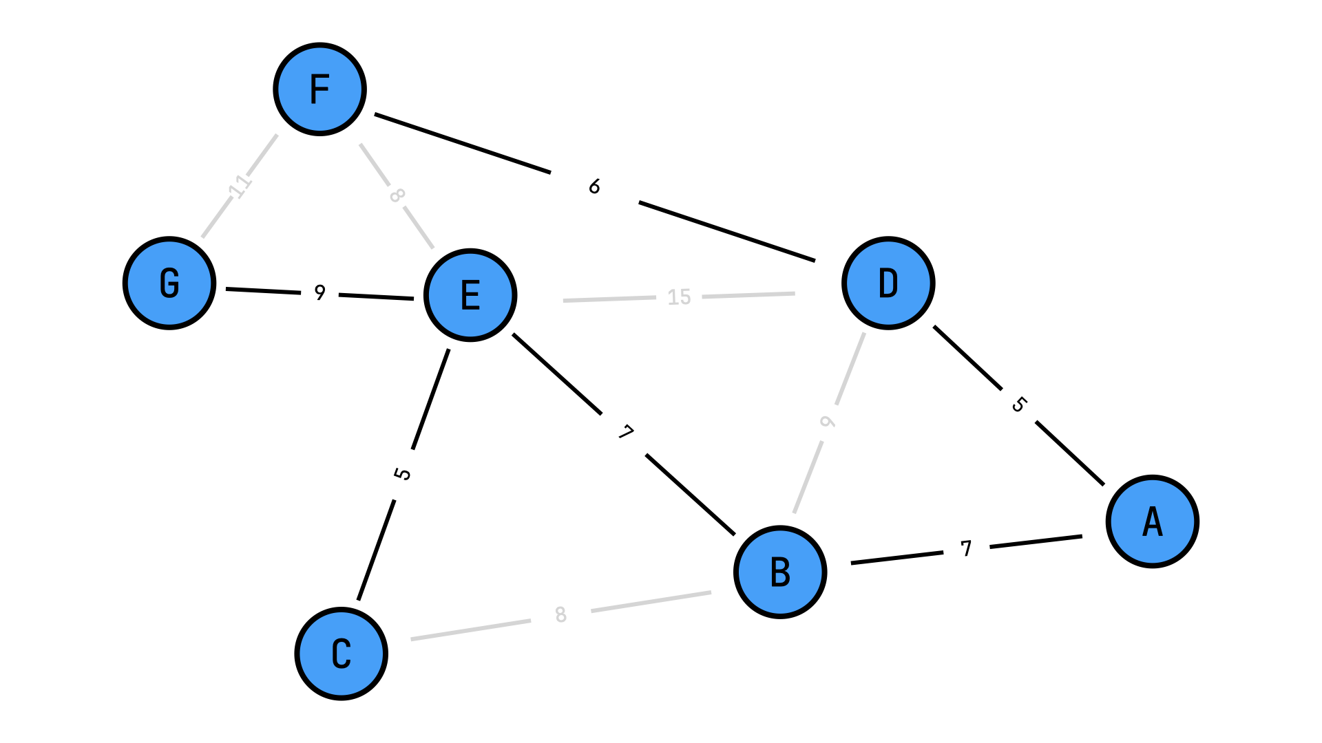

---

1. A quote from Ralf Hinze: Functional languages excel at wholemeal programming, a term coined by Geraint Jones. Wholemeal programming means to think big: work with an entire list, rather than a sequence of elements; develop a solution space, rather than an individual solution; imagine a graph, rather than a single path. The wholemeal approach often offers new insights or provides new perspectives on a given problem. It is nicely complemented by the idea of projective programming: first solve a more general problem, then extract the interesting bits and pieces by transforming the general program into more specialised ones.

   For example, consider this pseudocode in a C/Java-ish sort of language:

   int acc = 0;
   for ( int i = 0; i < lst.length; i++ ) {
     acc = acc + 3 * lst[i];
   }

   This code suffers from what Richard Bird refers to as indexitis: it has to worry about the low-level details of iterating over an array by keeping track of a current index. It also mixes together what can more usefully be thought of as two separate operations: multiplying every item in a list by 3, and summing the results. In Haskell, we can just write

   sum (map (3*) lst)

   ↩︎

2. Num is a typeclass which encompasses all numeric types of Haskell such as Int, Float, Double, etc. It defines e.g. how to add (+) and multiply (*) numbers. We will go into much more depth on typeclasses in future lectures. ↩︎